
Generative-inference models: Theory and empirical analysis (Part I)
The work presented in this blog is still in progress and summarizes my thesis’s chapters 3 and 4.
Foundation of generative-inference models
We will refer as generative-inference models to every model that considers a generative model $\boldsymbol{p}$ and an inference model $\boldsymbol{q}$. For these models, in general we will consider two variables: $\boldsymbol{x \in \mathcal{X}}$ and $\boldsymbol{z \in \mathcal{Z}}$, $\boldsymbol{\mathcal{X}}$ being the observable space and $\boldsymbol{\mathcal{Z}}$ being a latent low-dimensional manifold space.
When two variables are considered the joint distributions are $\boldsymbol{p(x,z)}$ and $\boldsymbol{q(x,z)}$. The generative model $\boldsymbol{p(x,z)=p(x|z)p(z)}$ is decomposed in a prior distribution $\boldsymbol{p(z)}$ and a decoder $\boldsymbol{p(x|z)}$ usually modeled as a neural network (NN). The inference model $\boldsymbol{q(x,z)=q(x)q(z|x)}$ is decomposed in the true underlying distribution of the data $\boldsymbol{q(x)}$ and an encoder $\boldsymbol{q(z|x)}$ usually modeled as a NN that codifies the data
In the following a diagram of the generative and inference models.
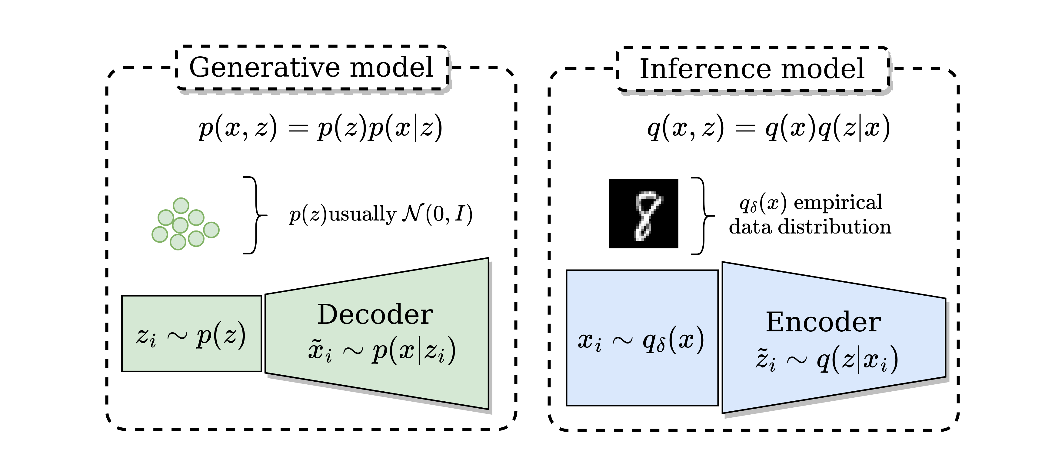 In the left hand size the generative model in green. In the right hand side, the inference model in blue.
As the generative-inference models have a generative model and an inference model we can expect them to have representation learning capablities as well as generative capabitilies. The following properties summarize this desired behaviour.
- Desired property 1. The marginal distributions of generative-inference models should match i.e. $q(z), p(z)$ should be equal and $p(x), q(x)$ should be equal.
- Desired property 2. Data $x_i \in \mathcal{X}$ sampled from the empirical data distribution $q_{\delta}(x)$ should have a high correlation with its codified version $z(x_i) \in \mathcal{Z}$ in the latent space.
Desired property 1 is a restriction given by the graphical models $p$ and $q$. The inferred marginal distribution $q(z)$ should follow the prior distribution $p(z)$, which can help for representation learning. For example, in MPCC, $\boldsymbol{p(z) = \sum_y^K p(z|y)p(y)}$ allowing clustering capablities. Additional the generated marginal distribution $p(x)$ should follow the real distribution $q(x)$ i.e the model generates realistic data.
Desired property 2 tells us about the representation learning capabilities of the model. If the codified version $z(x_i)$ of the data $x_i \sim q_{\delta}(x)$ is well represented in the latent space this would mean that a simpler classifier can be trained in the lower dimensional space $\mathcal{Z}$. We will study a mutual information perspective by bounding it with likelihoods $\mathbb{E}_{q(x)}[\log p(x|z)]$ or $\mathbb{E}_{p(z)}[\log q(z|x)]$, which is related with generative models as we will see in this post. This approach is different from previous work.
How to obtain desired properties 1 and 2.
Desired properties 1 and 2 can be achieved by matching the joint distributions $\boldsymbol{p(x,z)}$ and $\boldsymbol{q(x,z)}$. If the joint distributions are equal then:
- The marginal distributions $p(x)$, $q(x)$ and $q(z)$, $p(z)$ are equal too (desired property 1). This is easy to observe by integrating one variable i.e. $\int_z p(x,z) dz = \int_z q(x,z) dz \equiv p(x) = q(x)$ and $\int_x p(x,z) dx = \int_x q(x,z) dx \equiv p(z) = q(z)$.
- The conditionals distributions are also equivalent as we can observe mathematically $q(x,z)/q(z) = p(x,z)/p(z) \equiv q(x|z) = p(x|z)$ and $q(x,z)/q(x) = p(x,z)/p(x) \equiv q(z|x) = p(z|x)$. If this occurs using deterministic conditional distributions we would obtain perfect reconstructions as shown in BiGAN (desired property 2).
The literature shows two different ways of matching the joint distributions. The first way is by matching the joint distributions adversarially as shown in BiGAN, ALI or BigBiGAN. The second way is based on decomposing the matching of the joint distributions in simpler terms using KL divergence.
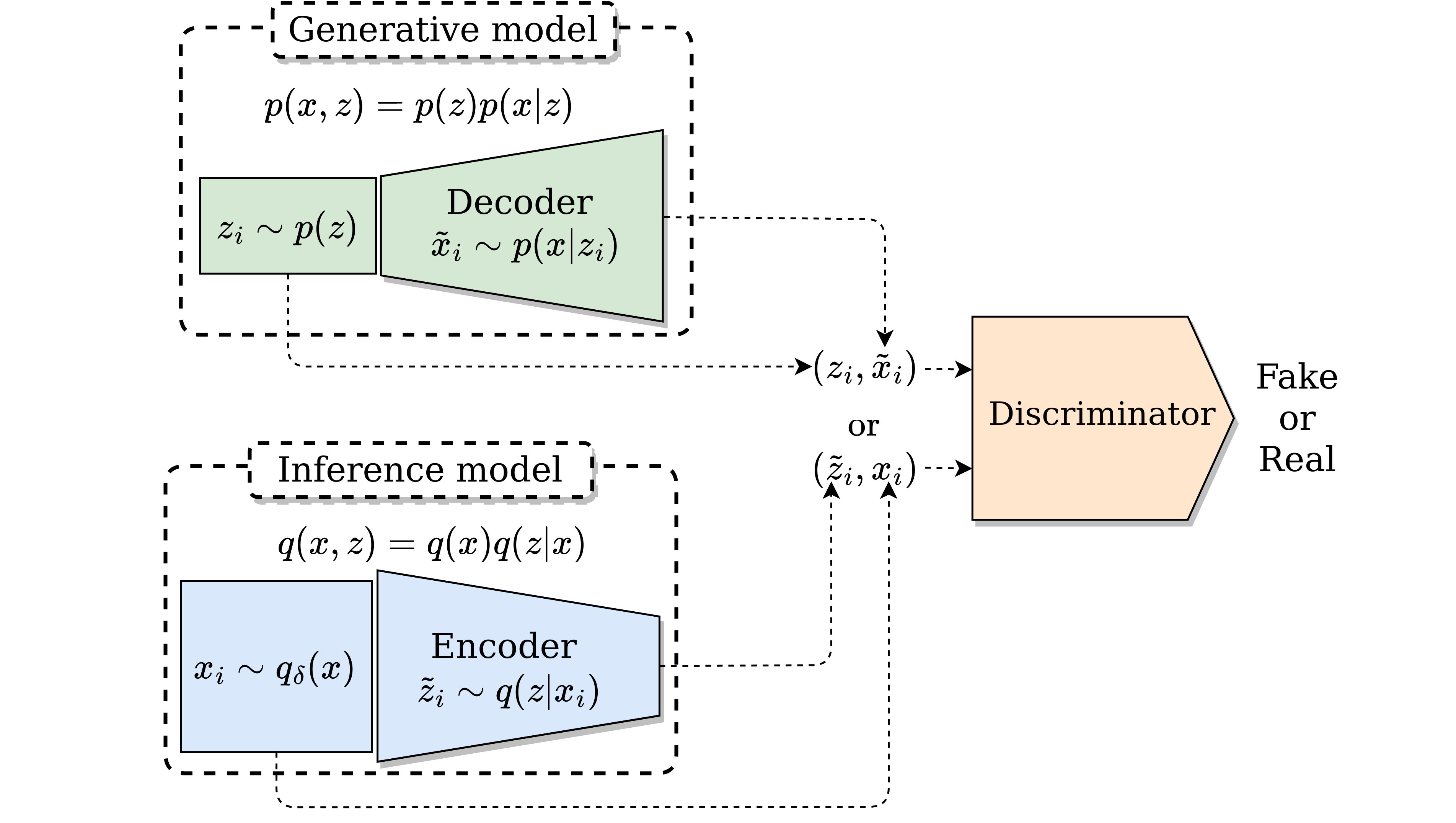
Matching $q(x,z)$ and $p(x,z)$ adversarially
The originally the objective of GANs is to match the marginal distribution $q(x)$ and $p(x)$ but it can be extended to match the joint distribution $q(x,z)$ and $p(x,z)$ as original done in BiGAN and ALI. The training is quite similar and have the same theoretical guaranties. A diagram of this type of training can be observed as follows.
Minimizing $D_{KL}(q(x,z)||p(x,z))$ by decomposing it
It also possible to math joint distribution by decomposing the KL divergence the model’s distribution.
We start by decomposing the KL divergence of the joints $q(x,z)$ and $p(x,z)$ as follows:
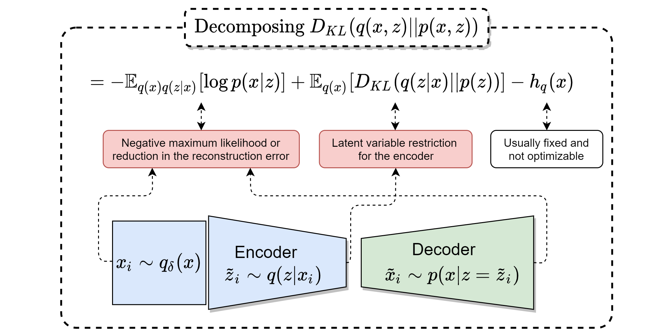
$$ D_{KL}(q(x,z) ||p(x,z)) ~~~~~~~~~~~~~~~~~~~~~~~~~~~~~~~~~~~~~~~~~~~~~~~~~~~~~~~~~~~~~~~~~~~~~~~~~ $$ $$ ~ = ~ \mathbb{E}_{q(x)} \mathbb{E}_{q(z|x)}[ - \log p(x|z) ] - h_q(x) + \mathbb{E}_{q(x)} [D_{KL}(q(z|x)|| p(z)) ]~~~~~~~~~ (1)~ $$ $$ ~ = ~ \mathbb{E}_{q(x)}\mathbb{E}_{q(z|x)}[ - \log p(x|z) ] - h_q(x) + \mathcal{I}_q(x,z) + D_{KL}(q(z)|| p(z) )~~~~~(2), $$
This divergence can be decomposed as in Eq. (1) or Eq. (2). Eq. (1) is optimized by Variational Autoencoders (VAE) with the exception of the entropy term $h_q(x)$. [$\beta$-VAE] and Adversarial Variational Bayes (AVB) also follow (1) modifying the optimization of $D_{KL}(q(z|x)||p(z))$, in particular [$\beta$-VAE] adds a constant to the KL-divergence term and AVB replaces it with adversarial training.
Other methods can be associated with (2) by replacing $D_{KL}(q(z)||p(z))$ with similar objectives. Info-VAE, Adversarial Autoencoders (AAEs), Wasserstein Autoencoders (WAEs) have followed this approach using adversarial training or maximum mean discrepancy between the marginal distributions. These models don’t explicitly optimize $\mathcal{I}_q(x,z)$ and thus the entropy term $h_q(z|x)$, which is included in $\mathcal{I}_q(x,z)$.
In the following, a diagram that encapsulates equation (1):
Minimizing $D_{KL}(p(x,z)||q(x,z))$ by decomposing it
We start by decomposing the KL divergence of the joints $p(x,z)$ and $q(x,z)$ as
$$ D_{KL}(p(x,z) ||q(x,z)) ~~~~~~~~~~~~~~~~~~~~~~~~~~~~~~~~~~~~~~~~~~~~~~~~~~~~~~~~~~~~~~~~~~~~~~~~~ $$ $$ ~ = ~ \mathbb{E}_{p(z)} \mathbb{E}_{p(x|z)}[ - \log q(z|x) ] - h_p(z) + \mathbb{E}_{p(z)} [D_{KL}(p(x|z)|| q(x)) ]~~~~~~~~~ (3)~ $$ $$ ~ = ~ \mathbb{E}_{p(z)}\mathbb{E}_{p(x|z)}[ - \log q(z|x) ] - h_p(z) + \mathcal{I}_p(x,z) + D_{KL}(p(x)|| q(x) )~~~~~(4), $$
The divergence $D_{KL}(p(x,z)||q(x,z))$ can be decomposed either as Eq. (3) or Eq. (4). Note that it is not possible to minimize $\mathbb{E}_{p(z)} [D_{KL}(p(x|z)|| q(x)) ]$, the third term of Eq. (3), using a closed form solution since we don’t have access to the $q(x)$ distribution. This could be optimized using adversarial training like AVB, but to the best of our knowledge this hasn’t been explored in the literature. However in practice Eq. (4) has been optimized in AIM or Info-GAN (if $c = z$).
Some final thoughts
In this blog I showed how the loss function of current generative-inference models can be obtained by using a joint distribution matching perspective. However, it doesn’t tell us anything about representation learning capabilities of the model. In the next blog we will expand more on this idea.