AGP: Amortized Gaussian Process
Amortized Gaussian Process (AGP) is a model that amortizes the computation of a Gaussian Process. With this model we can use autoencoders for time series with variable length and irregular time sampling. Note that while this model can be quite general we used it mainly for representation learning. Regression is one of our scopes for future research.
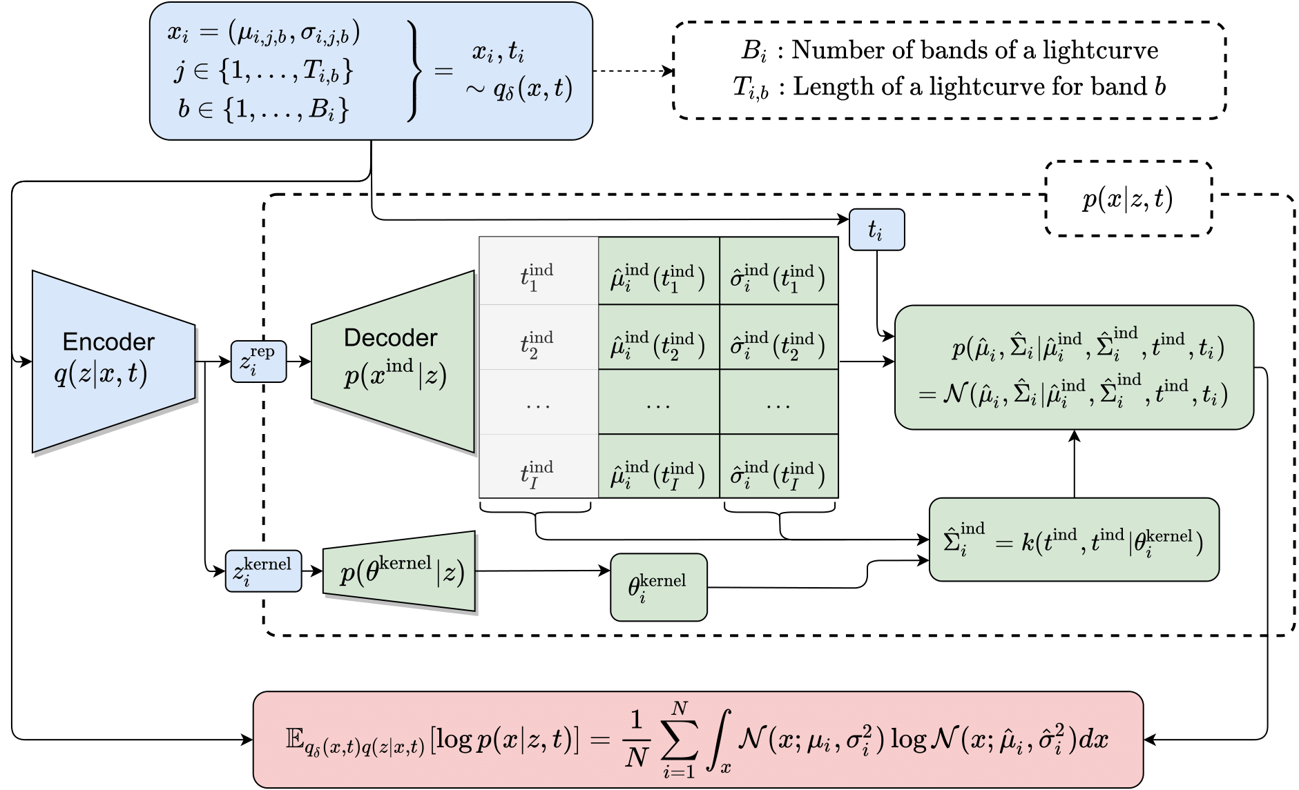
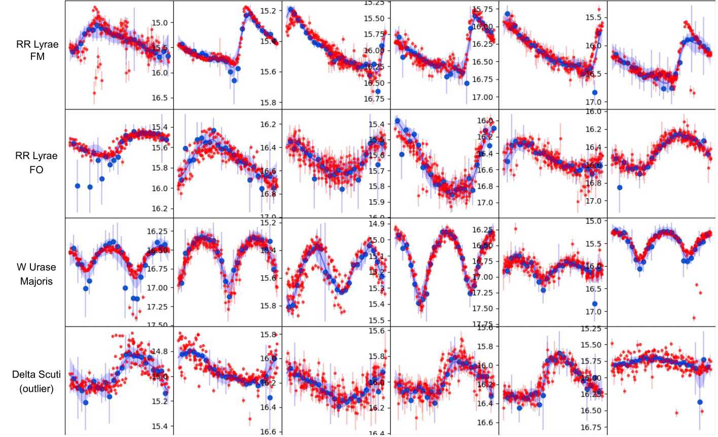
AGP is a decoder architecture that use a latent variable $\boldsymbol{z}$ (obtained by encoding some input $\boldsymbol{x}$) and decodes induction points and kernel parameters. With these two elements we can use a posterior distribution to make predictition in the observed space at all time space $\boldsymbol{t \in T}$. In the following image you can see the input data in red, induction points as blue circles and finally the prediction as a blue line.
Motivation
Autoencoder architectures are promising alternatives to train unsupervised or semi-supervised learning models in astroinfomatic. The amount of unlabeled data in astronomy is huge and unsupervised models like autoencoders are promising to explore. However, astronomical data are time series that have variable length and irregular sampling, so both the encoder and the decoder should deal with these difficulties. We proposed the decoder AGP for that purpose. In the following we explain the main methodology.
Methodology
This new decoder is motivated by Gaussian Process where the observed data $x_i, t_i \sim q(x, t)$ is used to predict points in the observable space at times $t^{\text{pred}}_i$ that do not correspond to the time distribution $q(t)$. This prediction is closed form for Gaussian distributions,
$$ p(A|B) = \mathcal{N}(\mu^{A|B}, \Sigma^{A|B}) \label{GaussianProcess} $$ $$ \mu^{A|B} = \mu^A + \Sigma^{A,B}(\Sigma^{B,B})^{-1}(\mu_{\text{data}} - \mu^B) $$ $$ \Sigma^{A|B} = \Sigma^{A,A} + \Sigma^{A,B}(\Sigma^{B,B})^{-1}\Sigma^{B,A}, $$
where in Gaussian processes $A$ refer to the predicted data, $B$ refer to the observed data and $\Sigma_{\theta_i}^{A,B}$ is a covariance matrix with dimension $|A|\times |B|$, constructed by a kernel function $k_{\theta_i}(\cdot, \cdot)$. Usually $\mu^A = 0$, $\mu^B = 0$. Note that is common to add in the diagonal of the covariance the data noise $\sigma_i(t_j)^2$ if it is considered.
Our proposed decoder is based on the contrary idea of Gaussian processes. Instead of assuming that the observed data generates a Gaussian process to predict data, we assume that exist an underlying process that generates the data.
This “underlying process” is estimated using an autoencoding procedure. We encode the available data into latent variables and we use a neural network decoder afterward that estimates the $B$ variables: $\mu_{\text{data}}$ estimated directly by the NN (this are the induction points as blue circles) and $\Sigma^{B,B}$, $\Sigma^{A,B}$, $\Sigma^{B,A}$ are constructed by estimating the parameters $\theta$ of the kernel function $k_{\theta_i}(\cdot, \cdot)$. These covariances along with $\mu_{\text{data}}$ are used to predict $\mu^{A|B}$ and $\Sigma^{A|B}$.
We use exponential quadratic kernel with parameters defined as $\theta_i^{\text{kernel}} = (\sigma_{\theta_i}, l_{\theta_i})$, estimated by $p(\theta^{\text{kernel}}|z)$ and learned through backpropagation.
$$ k_{\theta_i}(t, t^{\text{ind}}_j ) =\sigma_{\theta_i}^2 \exp \left(- \frac{||t-t^{\text{ind}}_j ||^2 }{2l_{\theta_i}^2}\right), $$
where $t^{\text{ind}}_j$ times are associated to fixed times (usually times regularly sampled in certain range, these times are the same for all data points $i$) and $t$ are the observed times. We additionally can estimate the noise of the covariance $\hat{\sigma}_{i}(t^{\text{ind}}_j))^2$ with a NN. We can obtain a posterior distribution that estimates the obervsed data $x$ at times $t$. Writting similar as before can obtained a closed form solution of such posterior distribution:
$$ p(\hat{x}| \hat{x}^{\text{ind}}, t^{\text{ind}}, t) = \mathcal{N}(\hat{\mu},\hat{\Sigma}) $$ $$ \hat{\mu}=\hat{\Sigma}^{\text{obs}, \text{ind}} (\hat{\Sigma}^{\text{ind}, \text{ind}})^{-1}\hat{\mu}^{\text{ind}} $$ $$ \hat{\Sigma} =\hat{\Sigma}^{\text{obs}, \text{obs}} - \hat{\Sigma}^{\text{obs}, \text{ind}} (\hat{\Sigma}^{\text{ind}, \text{ind}})^{-1}\hat{\Sigma}^{\text{ind}, \text{obs}} $$
Note we can maximize the likelihood of $p(\hat{x}| \hat{x}^{\text{ind}}, t^{\text{ind}}, t)$ (red box in the image below) using the observed data $x$.
The complete procedure should look something like this: