
MPCC: Matching priors and conditional for clustering
Clustering is a fundamental task in unsupervised learning that depends heavily on the data representation that is used. Deep generative models have appeared as a promising tool to learn informative low-dimensional data representations. In this blog we will dismitify MPCC, a generative model for clustering that we published on ECCV2020. [code]
Matching Priors and Conditionals for Clustering (MPCC) is a GAN-based model with an encoder to infer latent variables and cluster categories from data, and a flexible decoder to generate samples from a conditional latent space. MPCC is obtained through mathematical derivation and allows us to generate samples from different clusters in an unsupervised manner:
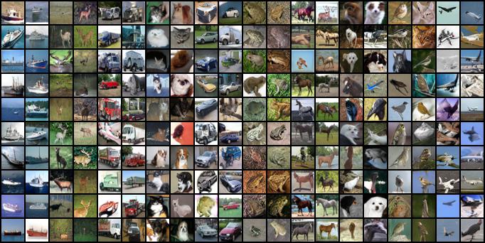 (Every two columns a different cluster)
Background
The idea of MPCC comes from a matching joint distribution optimization framework. To understand the intuition of what does it that means, let me denote some notation:
- Let $\boldsymbol{q(x)}$ be the true data distribution, where $x \in \mathcal{X}$ the observed variable.
- Let $\boldsymbol{p(z)}$ the prior of the latent distribution, where $z \in \mathcal{Z}$ the latent variable.
Let also define $\boldsymbol{q(x)}$ and $\boldsymbol{p(z)}$ as the marginalization of the inference model $\boldsymbol{q(x,z)}$ and generative model $\boldsymbol{p(x, z)}$ respectively. If the joint distributions $\boldsymbol{q(x,z)}$ and $\boldsymbol{p(x, z)}$ match then it is guaranteed that all the conditionals and marginals also match.
Intuitively this means that we can reach one domain starting from the other, i.e.:
-
If $\boldsymbol{p(z) \approx q(z) = \mathbb{E}_{q(x)}[q(z|x)]}$ we have an encoder, $\boldsymbol{q(z|x)}$, that allows us to reach the latent variables. In other words, $\boldsymbol{q(z)}$, the distribution obtained from all encoded observed data $\boldsymbol{x \in \mathcal{X}}$ should follow the prior $\boldsymbol{p(z)}$ that we established.
-
If $\boldsymbol{q(x) \approx p(x) = \mathbb{E}_{p(z)}[p(x|z)]}$ we have a decoder, $\boldsymbol{p(x|z)}$, that allows us to generate realistic data. In other words, $\boldsymbol{p(x)}$, the distribution obtained from all the decoded samples from the prior should follow the true data distribution $\boldsymbol{q(x)}$ that we established.
Previous works have also noted that VAE’s loss function can be obtained by expanding $\boldsymbol{D_{KL}(q(x,z)||p(x,z))}$. In this current work we analize more in depth what models can be obtained through this perspective. In MPCC, it is shown that VaDE can be obtained minimizing $\boldsymbol{D_{KL}(q(x,z)||p(x,z))}$, and in AIM models they showed a model obtained by minimizing $\boldsymbol{D_{KL}(p(x,z)||q(x,z))}$. MPCC borns from the motivation of minimizing $\boldsymbol{D_{KL}(p(x,z,y)||q(x,z,y))}$.
Before we continue, it is important to have an intuition of the advantages of three variable models ($\boldsymbol{x,z,y}$) over two variable models ($\boldsymbol{x,z}$). In three variable models we are assuming the existence of a third categorical latent variable $\boldsymbol{y}$ and a corresponding prior $\boldsymbol{p(y)}$. Since $\boldsymbol{y}$ is categorical, we are forcing the existence of an inference model $\boldsymbol{q(y|z)}$. In other words, we have an inference model that infers categories by encoding observed data $\boldsymbol{x \sim q(x)}$, and a generative model that generate realistic data by sampling from a categorical distribution $\boldsymbol{y \sim p(y)}$.
Matching priors and conditional for clustering
To derive MPCC, first we need to establish how the inference model $\boldsymbol{q(x,z,y)}$ and the generative models $\boldsymbol{p(x,z,y)}$ will be decomposed (the independence assumptions are explained in the paper).
- $\boldsymbol{q(x,z,y) = q(x)q(z|x)q(y|z)}$
- $\boldsymbol{p(x,z,y) = p(x|z,y)p(z|y)p(y)}$
In the paper we derived the following equality:
$$ \boldsymbol{\mathbb{E}_{p(x,z,y)}[D_{KL}(p(x,z,y)||q(x,z,y))}] ~~~~~~~~~~~~~~~~~~~~~~~~~~~~~~~~~~~~~~~~~~~~~~~~~~~~~~~$$ $$ = \underbrace{\mathbb{E}_{p(y)p(z|y)} [D_{KL}(p(x|z,y)||q(x))]}_{\textbf {Loss I} } + \underbrace{\mathbb{E}_{p(y)p(z|y)p(x|z,y)} [- \log q(z|x) - \log q(y|z) ]}_{\textbf{Loss II} } $$ $$ +~ \underbrace{\mathbb{E}_{p(z|y)p(y)}[\log p(y)+ \log p(z|y)]}_{\textbf{Loss III}} ~~~~~~~~~~~~~~~~~~~~~~~~~~~~~~~~~~~~~~~~~~~~~~~~~~~~~~~~~~~~~~~~~~~~~~~~ $$
The loss function of the right hand side can be minimized with closed form solution for the majority of their terms when assuming Gaussian distribution for $\boldsymbol{p(z|y)}$. Note that $\boldsymbol{p(z|y = c)}$ is basically a Gaussian for each cluster/categoy $\boldsymbol{c}$. And although they look quite criptic we can interpret them quite easily:
- Loss I: In the paper, we minimize $\boldsymbol{D_{KL}(p(x)||q(x))}$ adversarially instead of $\boldsymbol{D_{KL}(p(x|z,y)||q(x))}$. You probably think that minimize the first term instead fo the second is cheating but in my thesis we explore the differences between both measures. With this optimization we learn a decoder that aproximate the real distribution of the data.
- Loss II: Maximizing the likelihood $\boldsymbol{q(z|x = \tilde{x}_i)}$ is equivalent to train an encoder ($\boldsymbol{q(z|x)}$) that identifies the sample $\boldsymbol{z_i \sim p(z)}$ that generated $\boldsymbol{\tilde{x}_i}$. Maximizing the likelihood $\boldsymbol{q(y|z = z_i)}$ is equivalent to train a classifier ($\boldsymbol{q(y|z = z_i)}$) that identifies the sample $\boldsymbol{y_i \sim p(y)}$ that generates $\boldsymbol{z_i \sim p(z|y=y_i)}$. This last optimization separates each conditional distribution $\boldsymbol{p(z|y=c_k)}$ from the other, helping the clustering capabilities of the model.
- Loss III: These loss functions are basically entropies that help that latent varibles don’t collapse in local optimas.
Assumming Gaussian distribution for each conditional distribution $\boldsymbol{p(z|y=c) = \mathcal{N}(\mu_{c}, \sigma^2_{c}) }$, MPCC’s functioning can be observed as follows:
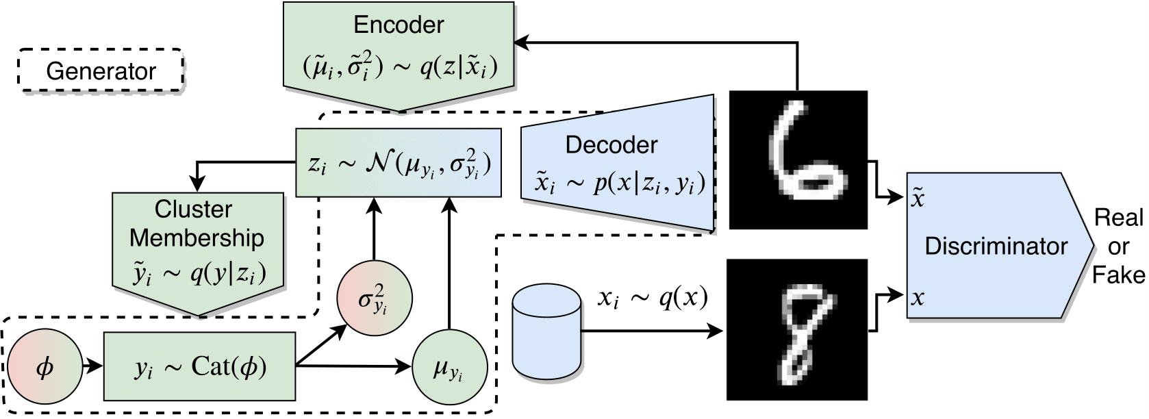 Fig 1: MPCC diagram components.
MPCC can also work for many clusters (CIFAR20 has 20 classes, and OMNIGLOT 100!) as we shown in the paper:
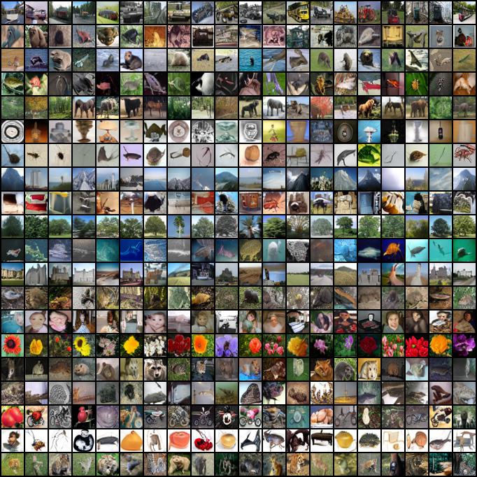 (Every row a different cluster)
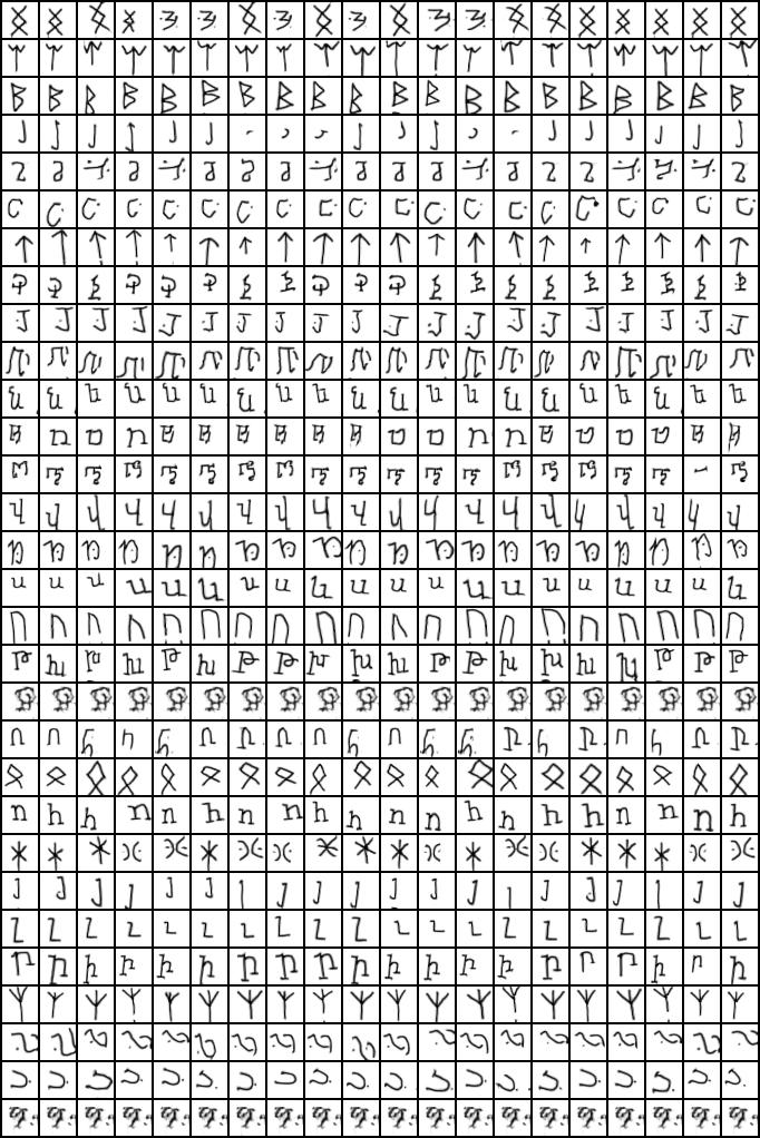 (Every row a different cluster)
For more results please refer to the paper.